
How does model training work?
In the previous series we trained a model to recognize different types of mushrooms, but what happened under the hood, how did it learn to do it. That is what we are going to learn today. There will be a bit of math to learn here, but its not complicated at all. So lets begin.
A simple example
Let’s start with the goal of trying to make it a goal to figure out the if a number is 15 or not. Of course this example is very trivial, its much easier to just create the algorithm: if(x == 15): return true, but the point of machine learning is toi have the machine learn how to do it rather than having to explicitly tell it how, which is much more difficult once we get into non-trivial examples, such as deciding what is a chanterelle mushroom and what is not.
So what do we need for this example? We need our labeled data of course, so lets start with a set of 10 numbers: 15, 72, 15, 31, 15, 1002, 15, 32, 15, 16. Not very much data and the correct number is always the same, as we will see this will lead to overtraining, but that is what we want in this case because there is only one true answer anyway. So the ground truth labels for each example is: true, false, true, false, true, false, true, false, true, false. Below is some notation we will use going forward:
nx = the number of features in each training example
x = an nx by 1 vector (array) of the features of a single training example
(x, y) = represents a training example, where x is defined above and y is the label, in this case it will be 0 or 1, true of false
m = the number of training examples
X = an nx by m matrix of all m training examples where each example x is a column of its features
Y = a 1 by m matrix containing the labels of each of the training examples.
For our example:
nx = 1, that is each training example has only one feature, the number itself.
x1 = 15, the superscript 1 here denotes which training example we are speaking of, x2 = [72], x3 = [15], x4 = [31], x5 = [15], x6 = [1002], x7 = [15], x8 = [32], x9 = [15], x10 = [16].
(x1, y1) = ([15], true), (x2, y2) = ([72], false), (x3, y3) = ([15], true), (x4, y4) = ([31], false), (x5, y5) = ([15], true), (x6, y6) = ([1002], false), (x7, y7) = ([15], true), (x8, y8) = ([32], false), (x9, y9) = ([15], true), (x10, y10) = ([16], false).
m = 10
X =
| x1 | x2 | x3 | x4 | x5 | x6 | x7 | x8 | x9 | x10 |
| 15 | 72 | 15 | 31 | 15 | 1002 | 15 | 32 | 15 | 16 |
Y =
| y1 | y2 | y3 | y4 | y5 | y6 | y7 | y8 | y9 | y10 |
| 1 | 0 | 1 | 0 | 1 | 0 | 1 | 0 | 1 | 0 |
Logistic Regression
Now, what we would like our model to do is that when we give it a number x as input, what will come out of that will be the prediction about whether x is 15 or not, lets call that ŷ, also known as y-hat, and should be a value between 0 and 1. For our parameters we have these two values which seem mysterious, w and b, where w is a nx dimensional matrix, and stands for “weights”, and b an integer that stands for “bias”. When we start our deep learning algorithm we don’t know the optimal values of these yet so we will start with either 0 or a random number depending on the type of network we are building. To get our prediction we will use the sigmoid function, represented by σ , applied to the formula, ŷ = wtX + b…
But hold on, if you are familiar with algebra, then this should look familiar, it simply y = mx + b, the equation of a line. As a refresher, y is the dependent variable, x is the independent variable and m is the slope of the line, and b is the y intercept, or where the line crosses the y axis. For those who are a little rusty lets do a quick example, lets plot the line y = x + 2, you can paste this into your python console to see the plot yourself as well here is the code and the plot:
import matplotlib.pyplot as plt
import numpy as np

# Create a range of x values
x = np.linspace(-10, 10, 400)

# Calculate y values
y = 1*x + 2

# Create a new figure
plt.figure()

# Plot x against y
plt.plot(x, y)

# Set the labels for x and y axes
plt.xlabel('x')
plt.ylabel('y')

# Set the title of the plot
plt.title('Plot of y = 1x + 2')

# Draw x and y axes
plt.axhline(0, color='black',linewidth=0.5)
plt.axvline(0, color='black',linewidth=0.5)
plt.grid(color = 'gray', linestyle = '--', linewidth = 0.5)

# Set the scale of the x and y axes to increment by 1
plt.xticks(np.arange(min(x), max(x)+1, 1))
plt.yticks(np.arange(min(y), max(y)+1, 1))

# Display the plot
plt.show()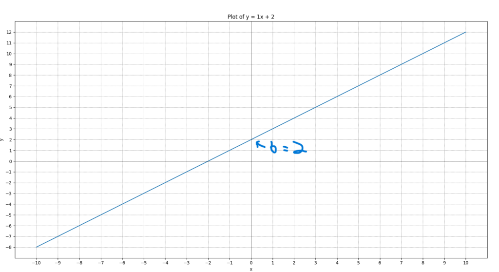
I’ve marked of b here which is 2, and as you can see, that is where it crosses the y axis, and the slope of the line is the “rise” over the “run”, which is to say to track the line, for this equation you go up one number then over one number and you end up on the next discrete point on the line, here it is, of course 1/1. And as you can see you can choose any x and get your y value, so for instance when you input x = 5 then you y = 7. Now that everyone is all caught up now we can ask the question: Why is it now “wtX+b” instead of mx+b, why the sigmoid function and what is the sigmoid function anyway?
Why wtx+b?
Firstly, let’s explain the superscript t, what is that? Well, that just means that we will need to transpose w so that we can perform a matrix multiplication called the dot product. Transposing is basically turning the rows of an array into its columns and its columns into rows, for the dot product to work they number of columns of the first array need to match the number of rows in the second column, like x, w has nx rows and 1 column, while X has nxrows and m columns so, (nx, 1) and (nx, m) respectively. In order to calculate the dot product we need for the number of columns in array 1 to match the number of rows in array to so we will basically lay array 1 on is side so that it now has the shape (1, nx) and we can perform the dot product operation.
What is the dot product and why use it?
This also gets into why we are using wtX+b instead of mx+b. In the case of the equation of a line, there is only a single feature, m and a single dependent variable x, when we are training our model generally there is more than one feature and more than one dependent variable (ie training example), so in order to get the slope of this multidimensional area we need to use the dot product of the slopes (weights) and the training examples. The dot product is created by taking an (a, b) sized matrix and multiplying its members with a (b, c) sized matrix such that we end up with an (a, c) sized matrix. Let’s say we have 2 matrices, matrix A which is of size, (1, 5) and matrix B which is of size (5, 3), the dot product is calculated as follows:
A = [a1, a2, a3, a4, a5]
B = [[b11, b12, b13],
[b21, b22, b23],
[b31, b32, b33],
[b41, b42, b43],
[b51, b52, b53]]
c1 = a1*b11 + a2*b21 + a3*b31 + a4*b41 + a5*b51
c2 = a1*b12 + a2*b22 + a3*b32 + a4*b42 + a5*b52
c3 = a1*b13 + a2*b23 + a3*b33 + a4*b43 + a5*b53
C = [c1, c2, c3]
The above is the manual way to do this, just so we understand how it works, but thankfully this can be done in python very easily by simply using the numpy dot function like so: y_hat = np.dot(w.T, X) + b. Easy as that!
Now that we know what’s happening, I’ll explain why this works. When we have the equation for a line, we already know the slope and the y intercept and we just plug in the x and we get our y, and we are done. In the logistic regression algorithm we don’t know the proper weights (slopes) or intercept (bias) when we begin. We are ultimately trying to get the model to learn if there is an appropriate mix of weights and a bias that can predict whether or not an item is what we are looking for or not, based on the patterns found in the data in out training examples.
Back to the sigmoid function
Now, with that out of the way, the next question is why do we need the sigmoid function and what is it? if we were to just use wtX+b our prediction could be really huge numbers, really small numbers, or large negative numbers, and if that is what we are left with how do we know what that means as far as a prediction? Enter the sigmoid function, here is the formula: σ(z) = 1 / (1 + e^(-z))
Here, z, is our formula wtx+b, you can try it out by on a calculator or in python using the np.exp function for euler’s number like so:
def sigmoid(z):
    return 1 / (1 + np.exp(-z))
What this will do is basically, if z is a large number the denominator will become 1 + a very small number, and the sigmoid function will end up being approximately 1/1, which of course equals 1. If z is a very small or negative number the denominator becomes large, and the value of the sigmoid function begins approaching 0. In this way we turn our prediction into a value between 0 and 1, which can be interpreted as a confidence metric, that is if y-hat is less than .5 it is considered to be 0, and if, for instance a prediction came out as 0 with a value of .49, that means that it is predicting that it is not what we are looking for, but is not very confident about the choice, where as if the value were . 001 it would be highly confident about it not being what we are looking for.
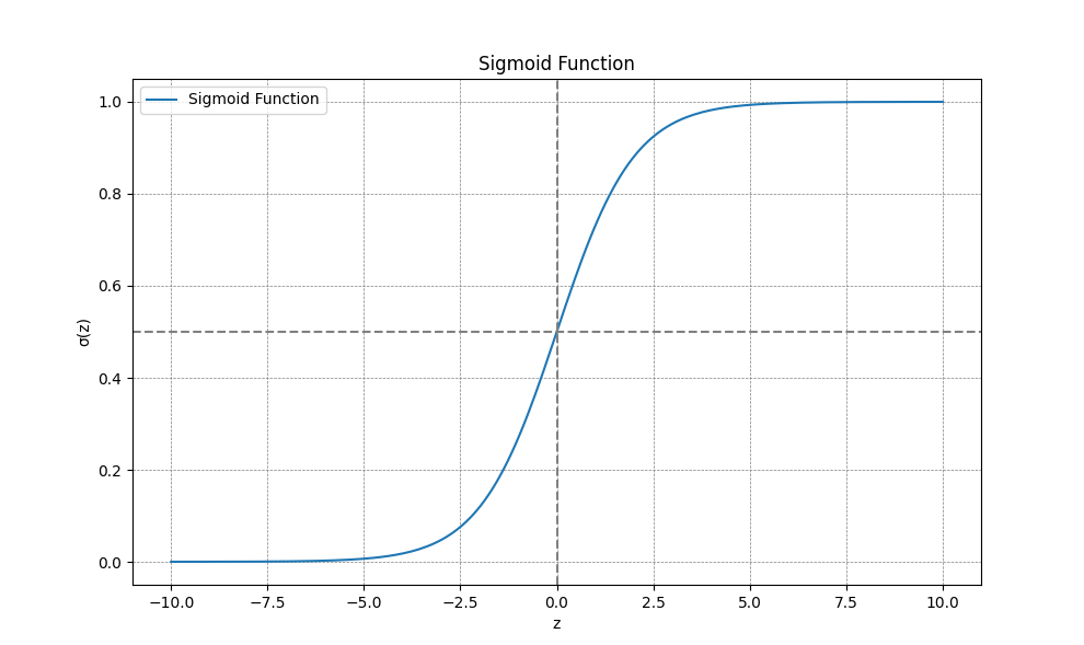
The above is the graph of the sigmoid function, and as you can see it gets it’s name due to the shape resembling an “s”.
We will end here for this installment. Now that we have arrived at this point we are ready to begin to understand the process of forward and backward propagation to improve our models predictive capabilities. See you next time!