With the recent advancement in AI technologies the last few years, it seems like the technology has touched almost every facet of our lives, but many don’t realize how easy it is to jump into the technology yourself and begin creating useful application quickly. No you don’t need an advanced degree in Machine Learning or Mathematics, though it would help if you do have some coding experience so that you know some of what you are looking at. You don’t even technically need a decent GPU since you can run on the CPU, although that will be much slower, so an NVidia graphics card is recommended.

Setting Up Your Environment

You’ll be either using an NVIDIA GPU or your CPU for the purposes of this tutorial.

1. Install or update your GPU drivers from the NVIDIA Driver Downloads page or from your GeForce Experience App.
2. Next, if you are using an NVIDIA GPU you will need to install the CUDA Toolkit.

Windows Installation Without WSL

1. You will need to install Python (Version 3.x is recommended.)
2. Install Conda (For creating seperate python environments): https://docs.conda.io/projects/conda/en/latest/user-guide/install/windows.html
3. Open the anaconda or miniconda app

Installing with WSL

I prefer to work in a linux environment, so I use WSL2. To do this you will need to add wsl to your system, install Ubuntu, and then install CUDA Toolkit for WSL

1. Install WSL2: https://learn.microsoft.com/en-us/windows/wsl/install
2. Install Ubuntu for WSL, follow the instructions for the following link but stop at step 4: https://ubuntu.com/tutorials/install-ubuntu-on-wsl2-on-windows-11-with-gui-support#4-configure-ubuntu
3. Open Ubuntu
4. Update the system: sudo apt update && sudo apt upgrade -y
5. Install python on Ubuntu: sudo apt install python3 python3-pip -y
6. Install Cuda Toolkit For WSL on Ubuntu: https://developer.nvidia.com/cuda-downloads?target_os=Linux&target_arch=x86_64&Distribution=WSL-Ubuntu&target_version=2.0&target_type=deb_local
   • Here you will get a list of commands based to execute in your linux distro mine are as follows:
     • wget https://developer.download.nvidia.com/compute/cuda/repos/wsl-ubuntu/x86_64/cuda-keyring_1.1-1_all.deb
     • sudo dpkg -i cuda-keyring_1.1-1_all.deb
     • sudo apt-get update
     • sudo apt-get -y install cuda-toolkit-12-3
7. Install Imagemagick For Ubuntu on Windows (in step 2 I told you to stop at step 4 of the ubuntu installation instructions, this is because for whatever reason I kept having issues getting x11 apps to work, but imagemagick worked like a charm) so that images will actually show when the code runs the .show function.
   • If you are using WSL2 then you will only need to run the command sudo apt install imagemagick
   • If you are using WSL1 then you will also need too install Vcxsrv on windows, you can follow the instructions here: https://jdhao.github.io/2019/02/16/pillow_show_image_on_wls/
8. Install Conda
   • wget https://repo.anaconda.com/miniconda/Miniconda3-latest-Linux-x86_64.sh
   • bash Miniconda3-latest-Linux-x86_64.sh
   • Restart Terminal
   • Initialize Conda. If you didn’t set it to automatically open, run the following command : conda init

Final Steps

These step are the same for either type of installation.

1. From your conda environment create a new environment: conda create --name pytorch-env python=3.8
2. Activate the new environment: conda activate pytorch-env
3. Install Pytorch using pip (make sure that you install the correct version based on the cuda version installed or CPU if you don’t have an NVIDIA GPU, you can check this by running the command: nvcc --version, (if you are running this in wsl to run this command you will need to navigate to /usr/local/cuda/bin, since it is not on the path), I have version 12.3, so I selected 12.1 on the following link.), get the proper command from here: https://pytorch.org/get-started/locally/ and then run it in your terminal

Check That the System is Properly Set Up

1. In your command line open up the python shell, by running the python or python3 command.
2. Then run the following:
   • import torch
   • print(torch.__version__)
   • print(torch.cuda.is_available())
3. If everything went well then you should get a response of True
   • If you got a false make sure that the cuda version installed and the version of pytorch match

Obtain Key For Bing Image Search

To make getting images for our training a bit easier we will start with using the Bing image search api to get some pictures of what we are training on from the internet. To access the api you will need to get a key, which you can do by following the instructions here: https://www.microsoft.com/en-us/bing/apis/bing-image-search-api. Make sure to sign up for the free tier.

That is probably the most difficult part, from here on it will be smooth sailing.

Clone the Project

We will step through a repo I created specifically for this tutorial.

1. Clone the repo: git clone git@github.com:ericsmallw/GettingStartedWithDeepLearning.git
2. Install all requirements for the app: pip install -r requirements.txt
3. Copy the .env-sample file and create a file named .env, and add your key for bing image search.
4. Check out the first step: git checkout step1

Step 1

So here were are, finally, ready to dive in. My family and I often like to go mushroom hunting for edible mushrooms in the forest, usually after a rain, you can sometimes find some really good treats such as chanterelle or chicken mushrooms, one problem though is that some, like the chanterelle have deadly look-a-likes. For the chanterelle, this deadly imposter is called the jack ‘o lantern, so called because it glows in the dark, but usually I’m mushroom hunting during the day, so if I’m not an expert it would be nice to have an app that could tell me the difference between the two. So that’s what we are going to build!

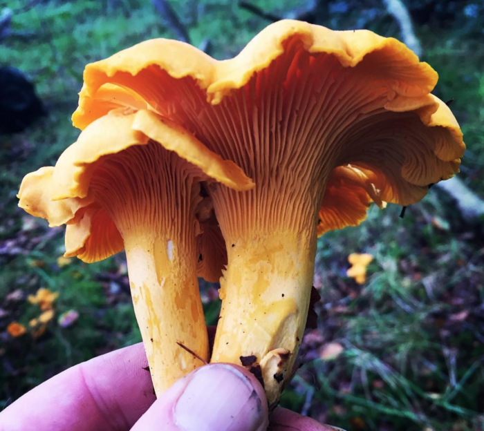
Chanterelle

Jack O’ Lantern

For this application we will make use of the fastai library which offers some very nice abstractions for pytorch that are very useful and save time when you are getting started with deep learning. This first step here will just be checking your azure key for the bing image search api.

def test_azure_key():
    results = search_images_bing(azure_key, 'mushroom')
    ims = results.attrgot('contentUrl')

    # print length of results to console
    print(len(ims))

    d = 'mushroom.jpg'
    download_url(ims[0], d)
    image = Image.open(d)
    resized_image = image.to_thumb(128, 128)
    resized_image.show()

Looking at the above code the search_images_bing function returns a list of urls from a bing search based on the supplied key word, and on the following line results.attrgot maps only the content urls of the results list to the ims variable. After that everything else is pretty straight forward, we take the first image in the list save it to the file “mushroom.jpg”, then resize the image to 128×128 px and then display it lets run it and make sure that works: python main.py

The Image that downloaded for me (yours may differ)

Let’s move on to step 2. git checkout step2

Step 2

This step is pretty much the same as the previous with a few more bells and whistles.

Starting with the main function, all I am doing here is passing a list of mushroom names to the get_images function, and after that is done it removes any png files from both folders since the training doesnt work with images that have transperency.

def main():
    mushroom_types = 'jack o\' lantern', 'chanterelle'
    get_images('images', mushroom_types)

    #remove any png files since they can have transparency
    remove_png_files('images/chanterelle')
    remove_png_files('images/jack o\' lantern')

The get_images function does just that, it iterates through the list of mushrooms and then gets 150 images of each, the bing api’s limit, then it will check to see if any of the images are broken and remove them.

def get_images(path_name, types):
    path = Path(path_name)
    if not path.exists():
        path.mkdir()

    for o in types:
        dest = (path / o)
        dest.mkdir(exist_ok=True)
        results = search_images_bing(azure_key, f'{o} {path_name}s')
        download_images(dest, urls=results.attrgot('contentUrl'))

    fns = get_image_files(path)
    print(fns)

    # remove any images that can't be opened
    failed = verify_images(fns)
    print(failed)
    failed.map(Path.unlink)

With that done let’s run that with python main.py move onto step3 and actually do some training! git checkout step3

Step 3

Here is where the magic happens, we will package our images so that they can be used to train a model. I’ve added a new function train_model:

def train_model(path):

mushrooms = DataBlock(
        blocks=(ImageBlock, CategoryBlock),
        get_items=get_image_files,
        splitter=RandomSplitter(valid_pct=0.2, seed=42),
        get_y=parent_label,
        item_tfms=RandomResizedCrop(224, min_scale=0.5),
        batch_tfms=aug_transforms()
    )

    dls = mushrooms.dataloaders(path, num_workers=0) # num_workers=0 to avoid a warning on windows

    learn = vision_learner(dls, resnet18, metrics=error_rate)
    learn.fine_tune(4)

    return learn

So, looking at this function we can see that we are creating a DataBlock, which is a blueprint for creating a DataLoaders object, which can be used to load training data in a way that is suitable for training a machine learning model.

In the DataBlock function call we can see that we specify the type of blocks it will be made up of (Image, because we are using images, and Categeory because it will be organized by category, specifically, the types of mushrooms we are checking for.

The get_items parameter takes a function, in this instance get_images, which tells it how to retrieve the data.

The splitter parameter defines how we will split the data in to the “training set” and the “validation set”, the training set is, in this case, the set of images we will use to train the model, and the validation set will be the set we will use to test the model. The value passed to splitter is a function that is set to pick 20% of the images from the dataset randomly and assign them to the validation set. The seed number is what determines which “random” images will be selected for the validation set.

Next up the get_y parameter defines how we will label our data, here I am using parent label, which means to use the items parent folder name for the category.

The item_tfms parameter sets the transforms for the image during each “epoch” or training pass, RandomResizedCrop will randomly select a portion of the image and crop and scale it to a specific size, in this case 244x244px. The larger the scale the better the result will be but it also makes the training slower and for the purpose of this model 244 is large enough. the mix scale parameter defines the minimum size the randomly cropped portion can be, in this case 50% of the image size. Each training pass will crop a different portion of the image, this will help prevent what is known as overfitting. To explain overfitting lets use an example with comedy, since that has been a hot topic in the news the past few days. Overfitting in deep learning is like when a comic works out his routine in a small area close to where he lives, he refines his jokes only based on that small local sample of people, and eventually he is doing really well and the local crowds love him, he then thinks its ready for the road, but when he travels from his small town to another city across the country the jokes fall flat. Similarly, a deep learning model overfits when it learns the training data too well, including noise and details that don’t generalize to new data. It performs impressively on the training data but poorly on new, unseen data because it fails to capture the broader patterns and instead has learned to recognize the specific examples it was trained on.

The final parameter in the datablock constructor is batch_tfms, which similar to item_tfms, will alter the images to give more variation and allow the model to be made more robust. These transforms include rotating, warping, zooming and lighting alterations that will differ during each epoch. Out of the box when using the aug_transforms function as the value of batch_tfms, will provide the transforms that generally work well with most models, but you can also provide parameters to control how the images are transformed if you’d like to.

In the next line we take the DataBlock we defined and create a DataLoader, which will break the data into the training and validation sets and get it ready to be processed by our learner which happens in the next line. (Note: setting the workers to more than 0 will speed up processing if you are using a non windows machine, on windows any value greater than 0 causes an error.)

Next, we finally get to defining our learner. Using the fast.ai library allows us to put this together fairly quickly, we define the type of learner we will be using, since we are want it to learn about images we will be using the vision_learner function, this function will take our DataLoaders object we just created, the next argument is what makes us able to train this model on our own machine rather than needing a server farm and millions of dollars to train our own model from scratch, we can load a pretrained model, in this case resnet18, a model with 18 layers trained on over 1 million images, and replace the last layer(s) with our own data specific to what we are trying to recognize. And finally we have the metrics we would like to evaluate the model and in this case we will use error_rate, which will tell us how often the model fails to categorize our images successfully.

Finally, we will run our training by calling learn.fine_tune, this function takes several parameters but for now we will only pass it one, a number representing number of epochs to train, here I am using 4.

Now, lets run it and see our results, run the command python main.py.

The first thing we will see is the results of the training in the console, here is what I got:

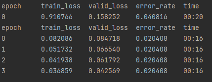
Those are great results! A bit too great, in fact for 2 mushrooms that look so similar, the important column to look at here is the error_rate, it goes from 4 percent to 2 percent and doesn’t change after that, which is odd behavior.

Next the learner gets returned and used in a function called examine_model where we take the modal we created and examine the results from our training:

def examine_model(model):
    interp = ClassificationInterpretation.from_learner(model)

    interp.plot_confusion_matrix()
    plt.show()

    interp.plot_top_losses(5, nrows=1)
    plt.show()

We simply pass our model into the fast.ai ClassifincationInterpretation.from function and then we can use the interpreter to see what we are looking at. The first image that will pop up is the confusion matric, mine looks like this:

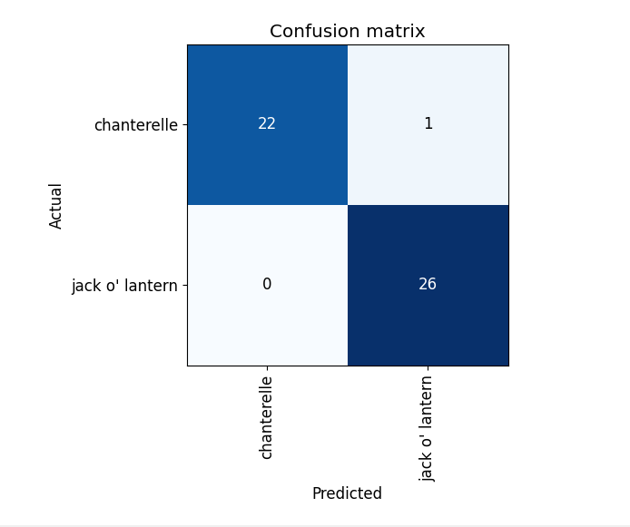
It got every classification correct except 1, which is still strange for such similar looking objects. Lets examine further. The next image that pops up displays top losses:

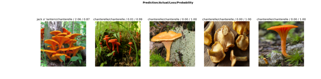
What this image shows is the prediction the model made for each image, the what the image’s category actually was, followed by what is essentially its confidence in its choice. loss is how uncertain it is, while probability is how certain it is that it is correct. As we can see in our Top Losses, only one image was actually incorrect, which matches our confusion matric, not only did it correctly guess everything else, but it was also nearly 100% confident in all of the predictions. I think we will need to check the images to see what going on a bit.

Lo’ and behold, the model was actually doing what it should have been doing, it can tell the difference easily because it is very easy to tell the difference between a chanterelle and whats in the jack o’ lantern folder:

No wonder it was so confident! Let’s go to the next step and fix this: git checkout step3.5

Step 3.5

To fix this I could search for the images as “jack ‘o lantern mushroom”, but I’m guessing that would still return some jack o’ lanterns so instead I’ll use its scientific name and change the main function as follows:

def main():
    mushroom_types = {'Omphalotus olearius'}
    # mushroom_types = 'jack o\' lantern', 'chanterelle'
    get_images('images/', mushroom_types)

    # remove_png_files('images/chanterelle')
    # remove_png_files('images/jack o\' lantern')
    remove_png_files('images/Omphalotus olearius')

    jack_o_lantern_path = Path('images/jack o\' lantern')
    try:
        for f in jack_o_lantern_path.ls():
            f.unlink()
    
        os.rmdir(jack_o_lantern_path)
        print(f"The directory {jack_o_lantern_path} has been deleted.")
    except OSError as e:
        print(f"Error: {e.strerror}")

    model = train_model('images')
    examine_model(model)

Here I’ve commented out the previous mushroom types and added only ‘Omphalotus olearius’, I then get those images, then remove any pngs and delete the old jack ‘o lantern folder, then train and examine again. Lets see how it turns out this time. Run the python main.py command again.

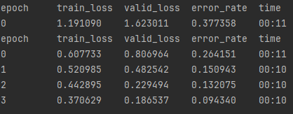
That is more like it, what we see here is the error rate starting at 38% then progressively getting better with each pass untill the 4th epoch where it ends at 9%.

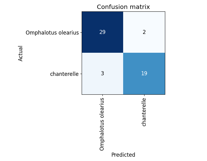
The confusion matrix also looks better now, the model guessed wrong a total of 5 times overall.

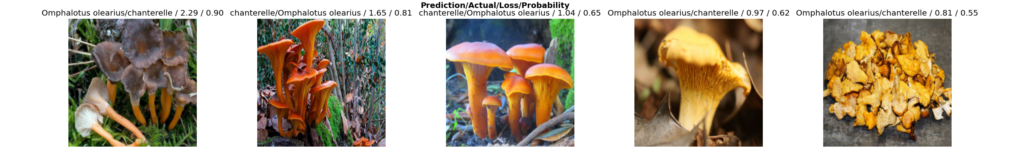
The Top Losses also looks better, there are now times when the predictions are lower than 90%.

While the model is pretty good, it can definitely be better, ideally we could get the error rate near 2%, and in the next part of this tutorial we will curate the data a bit and see what we can achieve.

Leave a message below if you have any questions, and of course try out any of your own ideas, and let me know what you come up with!